Sectoral Data: Demonstration¶

This section demonstrates the use of grants data, made available by 360Giving, to examine the extent to which organisations are connected to each other by sharing a common funder.

Guide to using this resource¶

This learning resource was built using Jupyter Notebook, an open-source software application that allows you to mix code, results and narrative in a single document. As Barba et al. (2019) espouse:

In a world where every subject matter can have a data-supported treatment, where computational devices are omnipresent and pervasive, the union of natural language and computation creates compelling communication and learning opportunities.

If you are familiar with Jupyter notebooks then skip ahead to the main content. Otherwise, the following is a quick guide to navigating and interacting with the notebook.

Interaction¶

You only need to execute the code that is contained in sections which are marked by In [].

To execute a cell, click or double-click the cell and press the Run button on the top toolbar (you can also use the keyboard shortcut Shift + Enter).

Try it for yourself:

print("Enter your name and press enter:")
name = input()
print("\r")
print("Hello {}, enjoy learning more about Python and SNA!".format(name))

Enter your name and press enter:

---------------------------------------------------------------------------
StdinNotImplementedError                  Traceback (most recent call last)
<ipython-input-1-0b0017c40e3d> in <module>
      1 print("Enter your name and press enter:")
----> 2 name = input()
      3 print("\r")
      4 print("Hello {}, enjoy learning more about Python and SNA!".format(name))

C:\ANACONDA3\lib\site-packages\ipykernel\kernelbase.py in raw_input(self, prompt)
    852         if not self._allow_stdin:
    853             raise StdinNotImplementedError(
--> 854                 "raw_input was called, but this frontend does not support input requests."
    855             )
    856         return self._input_request(str(prompt),

StdinNotImplementedError: raw_input was called, but this frontend does not support input requests.

Learn more¶

Jupyter notebooks provide rich, flexible features for conducting and documenting your data analysis workflow. To learn more about additional notebook features, we recommend working through some of the materials provided by Dani Arribas-Bel at the University of Liverpool.

Analysing networks of organisations¶

Preliminaries¶

In this section we import the Python modules we need for our analysis, as well as our network data set.

Python modules¶

import pandas as pd # data manipulation
import numpy as np # mathematical operations
import networkx as nx # network analysis
import matplotlib.pyplot as plt # data visualisation
from operator import itemgetter # suite of standard Python operators

Data set¶

We will use a dataset capturing connections between Manchester-based organisations in receipt of grants administered under the Covid-19 response scheme: https://covidtracker.threesixtygiving.org/

data = pd.read_csv("./data/manchester-org-network-covid19-2020-11-09.csv", index_col = 0)
data.iloc[:5, :5]

Each row is an organisation that received a grant (e.g., Greater Manchester Immigration Aid Unit (GMIAU)), each column also represents a given organisation, and each cell represents how many funders a pair of organisations both received a grant from. For example, two Manchester organisations would share a connection if they both received a grant from the same funder (e.g., Sport England). This may be useful information for an organisation to know, as it helps identify other organisations workign in the same space or on the same projects.

This is an example of an adjacency matrix: it maps who is next to whom in a social space. Saying two nodes are adjacent is another way of describing the presence of a tie between them. In addition we can also speak to the strength of the ties between funders: some jointly support 2 organisations, some jointly support 20 or more.

Therefore we have a valued, undirected network of organisations.

Finally, we are ready to convert the matrix into a networkx graph object:

fundgraph = nx.from_pandas_adjacency(data)
#print(nx.info(fundgraph))

Network-level measures¶

Visualisation¶

Visualising networks is an appealing activity and is often the first step in any analysis. However, as will become apparent, visualisation is an insufficient and often unrevealing output for all but the simplest networks (Hanneman and Riddle, 2005). For example, here is our network of Manchester organisations:

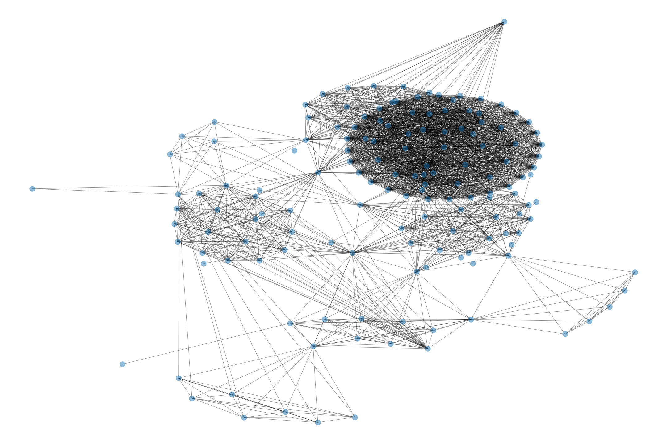
Organisation Network Random Layout

I’m sure you’ll agree that deriving insight on the essential properties of this network is difficult based on this visual representation. It is much better to dig into the mathematical measures for insight.

Size¶

Size is defined as the number of nodes and ties in a network. It is a simple and interesting measure in its own right, but it is also valuable for standardising other measures when we want to compare different networks.

print(nx.info(fundgraph))

There are 1964 ties (edges) between the 150 Manchester organisations. Average degree is a measure of the mean number of ties a node has with other nodes. In our example, an organisation is, on average, connected to 26 others through receiving grants from a limited number of funders.

Degree distribution¶

The distribution of the number of ties (degrees) in the network can be visualised using a historgram:

degrees = [fundgraph.degree(n) for n in fundgraph.nodes()]

plt.hist(degrees)
plt.title('Degree distribution')
plt.xlabel('Number of ties')
plt.ylabel('Number of organisations')

plt.show()

As you can see, there are a decent amount of connections between organisations in this network. For example, around 25 organisations are each connected to 25 others. While this seems like a lot of interconnection, remember the following: an organisation connected to 20 others does not mean that each pair receive grants from the same funder. Organisations A and B can receive grants from Funder 1, Organisations A and C receive grants from Funder 2 etc.

nx.number_of_isolates(fundgraph)

We see that there are eight organisations with no connections to others in the network: these are known as isolates. Basically these are organisations who receive grants a set of funders who do not support any other organisations in the network.

Density¶

How cohesive or dense is this network? That is, how many of the possible connections between organisations have been realised? We can use the nx.density() function to calculate a measure ranging from 1 (all connections realised) to 0 (no connections between nodes).

density = nx.density(fundgraph)
print("Network density:", density)

The network is reasonably dense - 18% of all possible ties between organisations are realised.

Node-level measures¶

Centrality¶

The centrality of a node is a measure of how it important it is in a network. A node may act as a hub, or broker connections between other nodes, or be positioned close to many other nodes. As such, there are difference measures of centrality we can apply to understand the importance of nodes.

Degree centrality¶

This measures how “popular” or well connected a node is in the network (Scott, 2017). It is a normalised measure of the number of ties a node possesses (usually direct ties but can be calculated at other distances).

First, let’s examine the raw number of ties each node has.

# Calculate number of degrees for each node and add as an attribute
degree_dict = dict(fundgraph.degree(fundgraph.nodes()))
nx.set_node_attributes(fundgraph, degree_dict, "degree")

# Sort by number of degrees and examine top 20 connected nodes
sorted_degree = sorted(degree_dict.items(), key=itemgetter(1), reverse=True)
print("Top 20 nodes by degree:")
for d in sorted_degree[:20]:
    print(d)

The best connected organisations are those receiving funding from Sport England (you can look up the identifiers using the 360Giving GrantNav tool.

Conclusion¶

Social Network Analysis (SNA) is a broad, rich and increasingly relevant methodology for investigating patterns in social structures and relations. There is a rich array of social concepts and constructs that can measured and analysed using social network data. This lesson demonstrated the use of some of these measures and techniques of analysis but there are many more to be discovered (see the networkx documentation).

Good luck on your data-driven travels!

Appendices¶

Calculating the size of a network¶

We can calculate the total number of possible ties in a network using a simple formula, which we adjust slightly depending on whether we are dealing with directed or undirected ties.

Directed ties¶

\begin{equation*} Y = n * (n - 1) \end{equation*}

Where Y = number of ties, and n = number of nodes

Undirected ties¶

\begin{equation*} Y = \frac{n * (n - 1)}{2} \end{equation*}